hary.oktav’s Blog

Plot continuous and discrete signal in Matlab December 13, 2008

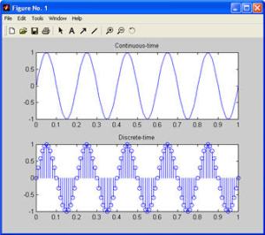
What is the difference of drawing continuous and discrete time signals? Sure, discrete signals are drawn with the matches-sticks-like to show the amplitude in a spacing-time to show the sampling rate. Whilst continuous signals are drawn continuously ^^. In Matlab, use PLOT command to draw a continuous signals. And use STEM command to draw discrete signals.

Drawing a continuous signal and discrete signal using MatLab.

Now for the code…

fs=100;						% sampling frequency
t=0:1/fs:1;					% setup time from 0 to 1 second
f=5;							% input frequency
x=sin(2*pi*f*t);			% input signal
subplot(211);plot(t,x);	% plot the signal
title('Continuous-time');
subplot(212);stem(t,x);	% plot the signal using stem
title('Discrete-time');

In my opinion, the way how those signals are drawn just the same. Both are actually discrete in time. There is a spacing-in-time defined by fs (sampling frequency). In continuous signals, lines are connected between two adjacent amplitudes. In discrete signals, each amplitude is disconnected by a-circle. So, I think this is different from the continuous-signal-in-a-real-world. In real world, there are no spacing-in-time for continuous signals. No way to define the sampling in continuous signals. Of course, sampling means to divide or to discrete (to separate, to disconnect)  the signals itself.

Discrete-time signal has aliasing concept, isn’t it? Aliasing means that if you do not proper in the way you sample a signal, then you will have a different signal from the origin. A different signal means that you will have a new signal in different frequency.

Now, try this. Change the f variable from 5 to 95. And run the program. You will see there is no different from previous figure. We expect that the more higher the frequency the more dense the signal. This is aliasing. The high frequency (95) signal looks like a low frequency (5) signal. Se, aliasing also happens on the continuous signal ^^ (in this case, of course).

Why? Since there is a sampling frequency (fs), it means that we threat a signals as a discrete-time signal. The sampling frequency  is 100Hz. Then, the nyquist frequency is 50Hz, a half from the sampling frequency. If you slowly change the f variable from 5 toward 50 then you will have denser signal. Beyond nyquist frequency (50 towards 100), everything is folding like a mirror: the signal become less dense.  So, we will expect that 5Hz and 95Hz look like the same as they are mirrored each other. Is that interesting enough? Yeap!