molecular sieve

Real molecules attract and repel each other. Ideal gas molecules don’t. That’s what causes nearly all deviations from ideality.

The ideal gas law is derived by ignoring attractions and repulsions between molecules. It doesn’t work at all for solids and liquids, which have very strong intermolecular forces. It generally isn’t accurate for real gases, either.

We can still apply the ideal gas law in the limit of low pressure for real gases. At low pressure, the gap between molecules widens, weakening the forces acting between molecules until they are essentially negligible, so the equation applies.

The Euler notebook posted below asks students to connect data for real gases collected at several different pressures with the ideal gas law by extrapolating to zero pressure. It introduces linear regression with Euler.

To use the notebook:

* Download and install the Euler Math Toolbox.
* Cut and paste the code below into a plain text file.
* Save the file with an .en file extension.
* Double-click the file. It should open up in the Toolbox.

I used this in my Fall ‘09 PChem class (it’s the fourth notebook in the series). Italics mark the items students had to fill in themselves. They seemed to have little trouble with this one.

All of the notebooks in this series are specifically keyed to Atkins’ Physical Chemistry, 8th edition.

—————————-snip here———————————————
% Notebook 1.3: Extrapolation to zero pressure
%
% In this notebook, we’ll calculate properties of real gases from the
% ideal gas law by extrapolating to zero pressure.
%
% Consider the following experimental data collected for gaseous
% dimethyl ether at 25 degrees Celsius. The pressures P are in pascals,
% and the densities d are in kg m^-3. R is in Pa m^3/mol K and T is
% K.
%
>P = [12.223,25.20,36.97,60.37,85.23,101.3]*1000;
>d = [0.225,0.456,0.664,1.062,1.468,1.734];
>R = 8.314;
>T = 25 + 273.15;
%
% Let’s find the molar mass of dimethyl ether from this data.
%
% The molar mass M of an ideal gas is mass per mole. The mass of the gas
% is its density times its volume, so
%
% M = dV/n
%
% For an ideal gas, PV=nRT or V/n = RT/P, so
%
% M = dRT/P
%
% The ideal gas law holds when P approaches zero, so for a real gas,
%
% M = lim dRT/P
% P->0
%
% This is called a limiting law. How can we apply the limiting law with the
% pressure and density measurements in P and d?
%
% First, calculate an array of dRT/P values.
%
>dRToverP = d*R*T/P;
%
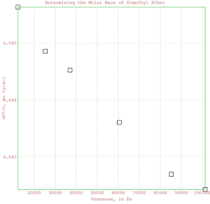
% Let’s plot these values against P to see if we can linearly extrapolate
% them to zero.
% * When plotting experimental data, it is good practice to show
% the points on the graph (use the points=1 option).
%
>plot2d(P,dRToverP,points=1,style=”[]”);
>title(“Determining the Molar Mass of Dimethyl Ether”);
>xlabel(“Pressure, in Pa”);
>ylabel(“dRT/P, in kg/mol”);
>insimg;

%
% The data looks reasonably linear. It’s worth trying to fit a
% line to it. We can use Euler’s polyfit() function to do this. The
% call looks like
% a = polyfit(x,y,n)
% where:
%
% a is an array of coefficients in the fitted polynomial
% a[1] + a[2]*x + a[3]*x^2 + … + a[n+1]*x^n
% x and y are the arrays of x and y data
% n is the degree of the polynomial to fit (1 for a line)
%
>fit = polyfit(P,dRToverP,1)
0.04587503092209 -3.583072735655e-008
%
% The first number is the intercept; the second is the slope.
%
% To calculate an array of points along the regression line, use the
% polyval() function. The call looks like
% y = polyval(a,x)
% where x, y, and a have been defined above.
%
>x = [0,max(P)];
>y = polyval(fit,x);
%
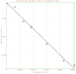
% Now insert the plot, with the raw data points marked as boxes,
% and the regression line displayed as a solid line.
%
>plot2d(x,y);
>plot2d(P,dRToverP,points=1,style=”[]”,add=1);
>title(“Determining the Molar Mass of Dimethyl Ether”);
>xlabel(“Pressure, in Pa”);
>ylabel(“dRT/P, in kg/mol”);
%
% The y-intercept is M, the value of dRT/P at P=0.
%
>M = fit[1]
0.04587503092209
%
% We can label the y-intercept using the label function. The call
% looks like label(text,x,y,offset). You can play around with the
% offset parameter until the label is where you want it.
%
>label(“M”,0,M,0);
>insimg;

% —————————————————————–
%
% Apply these techniques to solve problem 1.3 in the text, which
% finds absolute zero on the Celsius temperature
% scale from experimental data.
%
% Enter the P and alpha data in the space below.
% (HINT: look carefully at the units.)
%
>P = [749.7, 599.6, 333.1, 98.6];
>alpha = [3.6717, 3.6697, 3.6665,3.6643]*1e-3;
%
% It will be easiest to find alpha for an ideal gas first.
% Do this with the polyfit() function in the space below.
% Call the alpha value for an ideal gas ‘alphaideal’.
>fit = polyfit(P,alpha,1)
0.003662977448051 1.139259281072e-008
>alphaideal = fit[1];
%
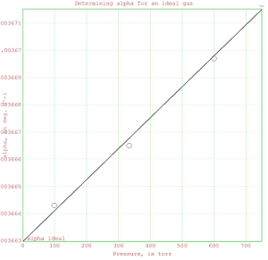
% In the space below, insert a plot that extrapolates alpha to zero
% pressure. Mark the data on the line as circles (use style=”o”) and
% add a regression line to the plot. The y-intercept should be shown
% and labeled as “alpha ideal”.
%
>x = [0,max(P)];
>y = polyval(fit,x);
>plot2d(x,y);
>plot2d(P,alpha,points=1,style=”o”,add=1);
>title(“Determining alpha for an ideal gas”);
>xlabel(“Pressure, in torr”);
>ylabel(“alpha, in deg. C^-1″);
>label(” alpha ideal”,20,fit[1],-25);
>insimg;

%
% Now solve Charles’ Law in the form V=Vo(1+alpha*theta) for
% absolute zero. Call the solution ‘absolutezero’.
% HINT: You won’t need an actual value for Vo, if you do your
% algebra correctly.
% HINT: At V=0, theta is absolute zero on the Celsius scale.
% HINT: Charles’ Law applies exactly only to ideal gases.
%
>absolutezero = -1/alphaideal
-273.0019537882
%
% ———————————————————————–
%
% Apply these techniques again to solve problem 1.7(b) in the text,
% which estimates the value of the ideal gas law constant R from
% experimental data.
%
% Enter the P, V, and density(d) data in the space below.
%
>P = [0.750000, 0.500000, 0.250000];
>V = [29.9649, 44.8090, 89.6384];
>d = [1.07144, 0.714110, 0.356975];
%
% Calculate an array of R values calculated at each of the three points.
% Call it RP (for “R at pressure P”).
%
>M = 2*15.9994;
>T = 273.15;
>RP = P*M/(d*T);
%
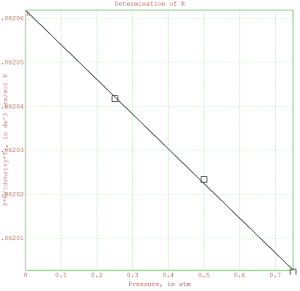
% In the space below, insert a plot of the RP values as a function
% of pressure. Show the data points as boxes (use style=”[]”). Draw
% the regression line on the plot. AS ALWAYS title the plot and
% label the axes. The axis labels should include the units.
%
>fit = polyfit(P,RP,1)
0.08206187029697 -7.886858741291e-005
>x = [0,max(P)];
>y = polyval(fit,x);
>plot2d(x,y);
>plot2d(P,RP,points=1,style=”[]”,add=1);
>title(“Determination of R”);
>xlabel(“Pressure, in atm”);
>ylabel(“P*M/(density*T), in dm^3 atm/mol K”);
>label(“R”,0,fit[1],0);
>insimg;

%
% In the space below, print your calculated R value.
>R = fit[1]
0.08206187029697